
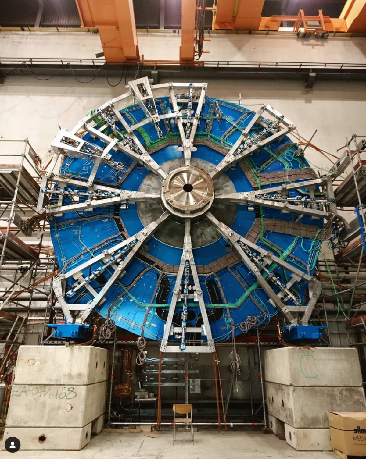
The ATLAS new small wheel detector (yes, the small one). After we upgrade the LHC in 2024, the collision rates and corresponding data rates are too high for our current detectors to handle. In order to keep data rates at a manageable level, ATLAS is improving their muon detectors to better discriminate between collisions which are interesting and those which are not.
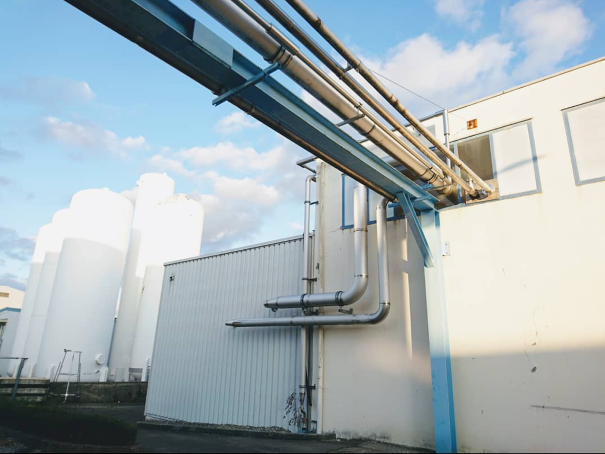
The CERN water tower
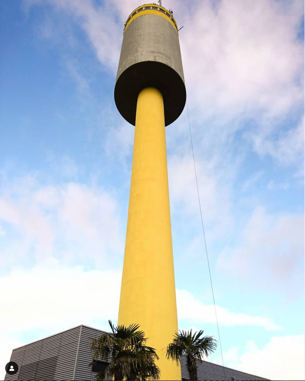
The water tower. Located at CERNs highest point, it holds 750 meters cube of water. We mainly use water as a coolant for the different facilities.
Moving CMS
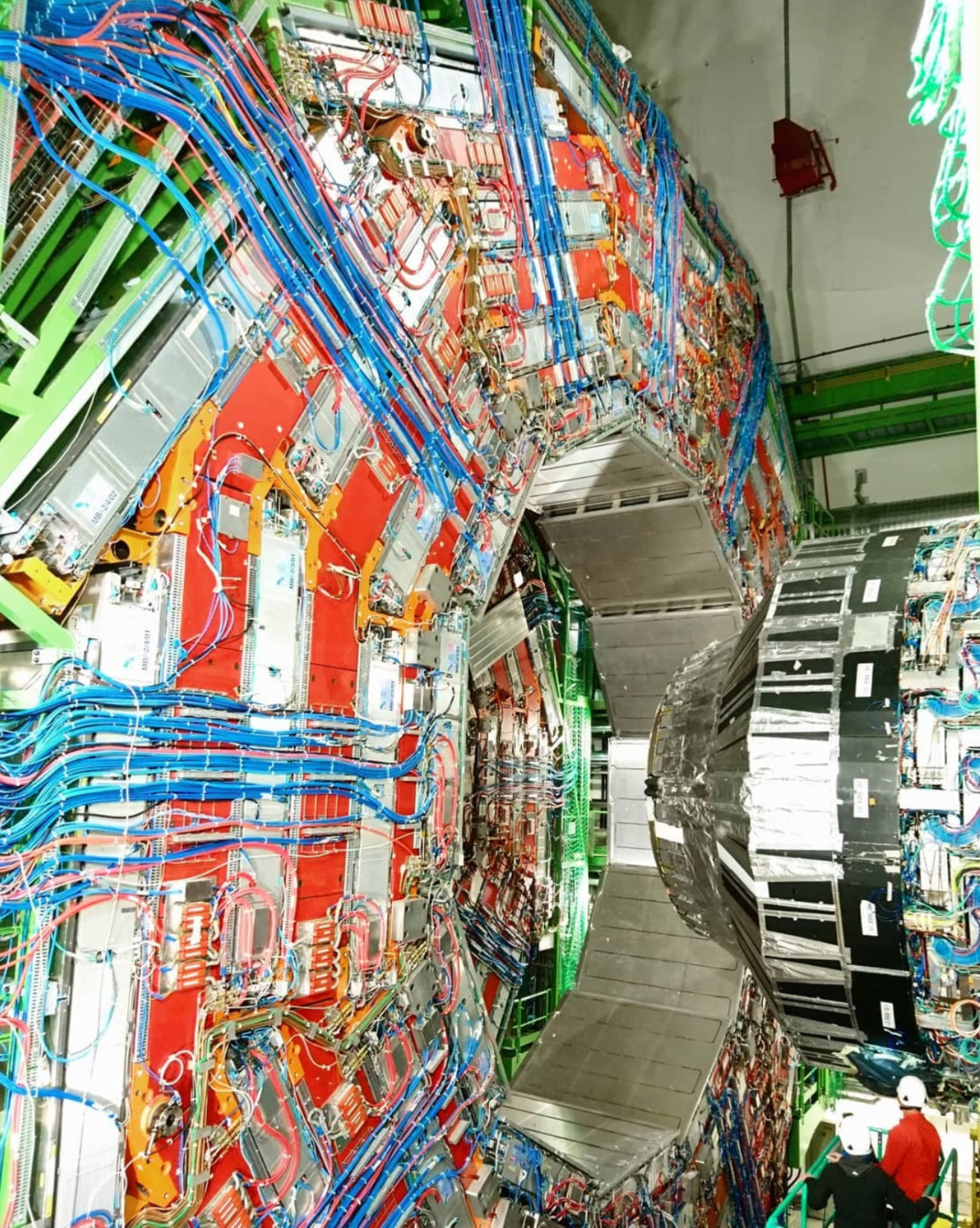
Today at the @cmsexperiment. The red structure is one slice of our barrel steel return yoke, there to control the magnetic field. We move it around using air pads, where compressed air (at 24 atmospheres) is pumped into little disks under its feet, causing it to float 1 cm above ground. In ten minutes, we can move it roughly one meter. Humans added for reference.
The CMS high-granularity calorimeter
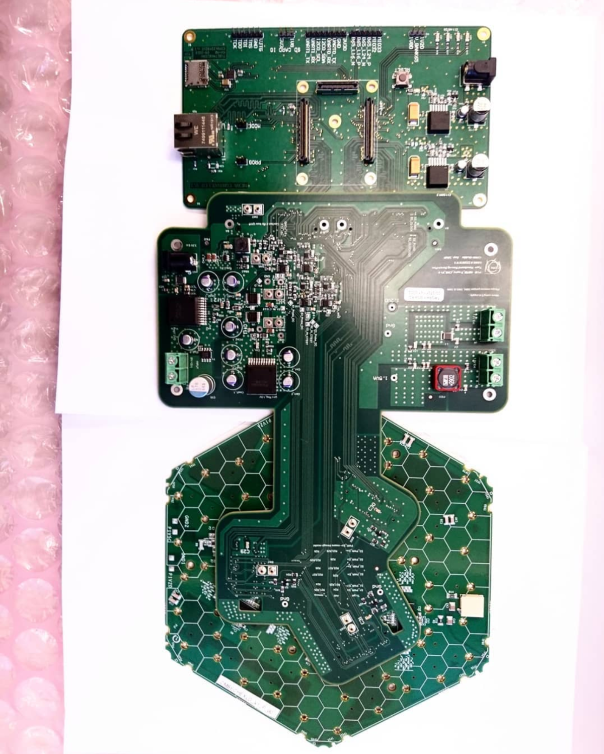
Our new hexagonal high-granularity calorimeter sensor, second and final(?) version (with testing board). Each little white hexagon represents a silicon crystal sensor, used to measure energy deposits of particles traversing the calorimeter volume. Each hole, a special design, connects three hexagons to the green printed circuit board through tiny wires @cmsexperiment
Research fellowship at CERN
As a research fellow you get three weeks to chat with the spokesperson of each CERN experiment, then freely choose where you want to do research(!!!) . My little nerd heart is literally exploding of excitement over how cool all of these experiments are. Here behind ISOLDE, which produces and studies radioactive nuclei
Every day battles
Where did I put the wifi password?
Big data
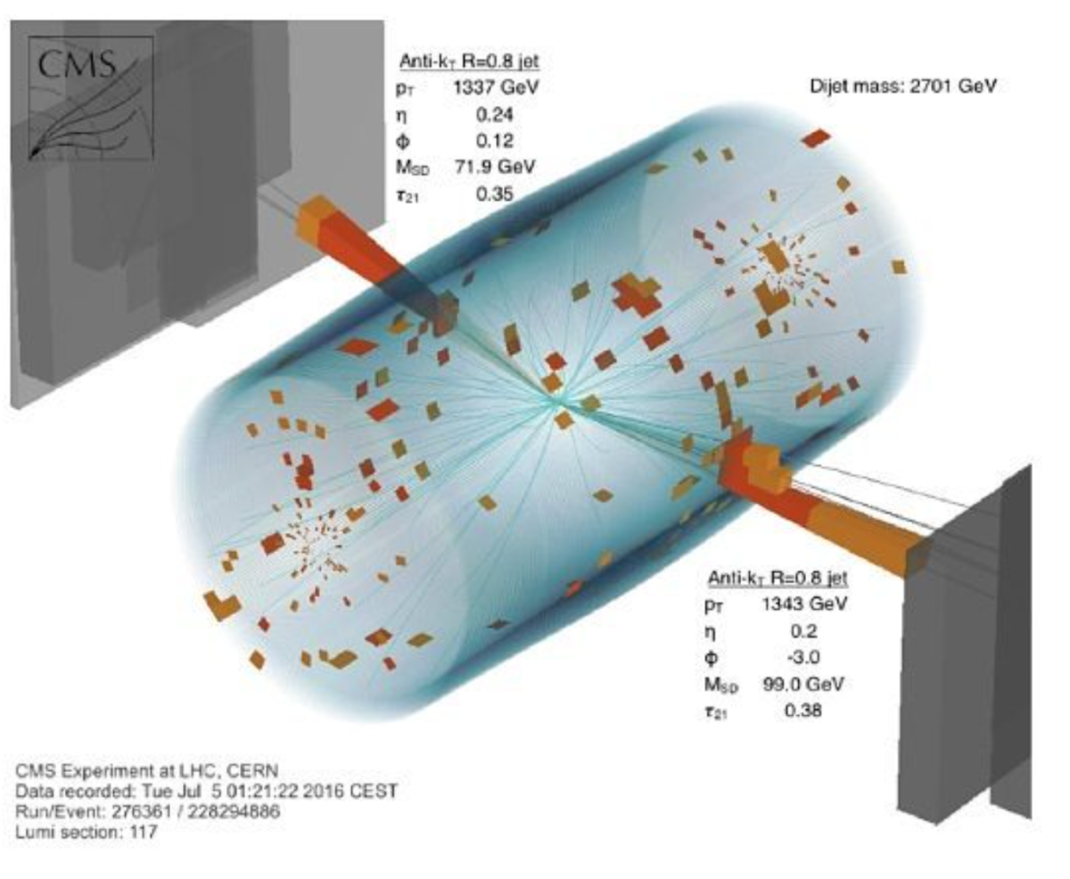
In ONE HOUR of LHC running we’ve produced roughly 180 Terabytes of data. That’s 7 years of HD video. Or, if you will, 20 Terabytes more than the entire Netflix library. One of the funner parts of my job is creating displays of real events that take place in our detector, like this one! (In total, we’ve collected over 200 petabytes, roughly 1400 years of HD video) #mycameraisbiggerthanyours
No-loose theorem

There is an interesting theorem in particle physics we call the no-lose theorem. It goes something like this: Say you have a theory and say someone is putting up an experiment to test your theory. If your theory fulfils the no-loose theorem, then ANY outcome of the experiment, is GUARANTEED to result in a new discovery. There is just no way you can loose (hence the name). The no-lose theorem came up around the time we were thinking about whether or not to build the Large Hadron Collider. Now, trying to convince ourselves as well as politicians in the early 1980’s that building a 27 km long ring at a 100 meter depth (rocky depth mind you) is an ok way to spend eight billion Euros required some pretty tangible arguments. Luckily we had one. The Standard Model of particle physics was at the time, and still is, the best model we have that describes the fundamental particles of nature and how they interact with one other. It had been amazingly successful in describing a wide range of phenomena as well as precisely predicting others. There was simply no end to its success. HOWEVER. As it was, the theory failed to predict how the fundamental particles of nature got their mass. There was something missing in the maths somewhere. Independently, Peter Higgs, Francoise Englert and Robert Brout came up with a solution to the problem, and with this, the final prediction of the theory: a spin-0 (see later post!) vector boson with an unpredicted mass, the so-called Higgs Boson.
The no-lose theorem was as follows: to keep our Standard Model from breaking down, there either had to be a Higgs Boson (with a mass below 800 GeV, more on that later), or something more interesting. A discovery of some sort or another was guaranteed if we had a machine capable of probing energies up to 1000 GeV
That’s why we started working on the LHC and why it was built to look for particles with masses up to 1 TeV.
Today, post-Higgs, there are no guaranteed discoveries anymore and we’re in somewhat of a “post-Higgs depression”. We know that the Standard Model, as it stands today, fails to describe all the phenomena we observe in nature; gravity, neutrino masses, the huge difference between the electroweak and Planck scale. So what’s next?
There is luckily one last no-loose theorem. And it’s origin is gravity. Stay tuned.
Part 1: From logistic regression to deep neural networks
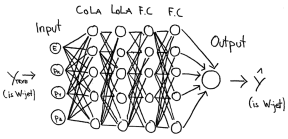
You’ve probably often heard that machine learning is a big black box that does some hocus pocus and then realistic images of people pop out. In this post, I’ll try to explain how deep neural networks (at least feed forward sequential ones) are actually quite straight forward and easy to understand.
It all begins with logistic regression. Let’s say you want to find a picture of your dog on your phone. Wouldn’t it be nice if your phone roughly knew what your dog looked like and could return you all pictures that contains images of your dog that you have on your phone? But how does a computer learn to tell the difference between a picture of your dog and a picture of your mom? All images are built up by pixels and each pixel can be a mixture of three colors: red, green and blue. Say you have a 64×64 pixel image of your dog and one of your mom. As a computer can’t “see” a picture it needs that input in words it can understand. So in this case, we make a vector of all the input features 


Let’s start by doing this in logistic regression. To go from the feature vector 

where you want 


The sigmoid function is

and looks like this

From this formula we can see that if 

So given this, the job of your computer or you is to properly estimate the weights in the matrix w and the bias b so that
Now how do we learn w and b? In order to do so we need to define a loss function, a measure of how close

We want this to be as small as possible because: If y=1 we want 
So we have our estimate for our estimator for ONE training sample, or if you wish, one picture of your dog. BUT we need multiple pictures of your dog in order to properly tune the parameters $w$ and $b$, some of your dog sleeping, some where he’s joyfulling skipping around, some where he’s from his bad side etc. In order to estimate the loss for all our training samples we define the cost function:


where the sum is over all your training samples.
SO. Your loss function is applied to a single training sample whereas the cost function is the cost of your parameters. So we want to minimzie the cost function J, by tuning w and b
Now, on to a very important concept in machine learning: gradient descent.

We want to change the weights w and the bias b such that J reaches a minimum. In order to find function minima and maxima, we use derivates. In praxis, we keep updating w and b in the following way:


where 
Wait. Stop! I’m bored for now. Will take a break and write a post on the CMS trigger. See you soon!
OK, its 6:05 and I’m on the morning train to CERN. Time for some ML!
So the key equation in DNN: Gradient descent. This holds for logistic regression and DNNs. FIrst, lets look at the example where you have one training sample, and look at how we have to change the weights with respect to the loss function L (remember, if we have multiple training samples as for a DNN, we need to change the weights with respect to the cost function J. We’ll get to this below)
Now remember we had the three following equations for the updates of x, the estimation of y,


Lets say we have two features, then we have


The derivative of the loss function with respect to a is:

And with respect to z

Once we have the derivatives, the final sep is to figure out how much we need to change w and b in order to get closer to the minimum. That means we need


These are the following:


So the updates to the weights are then


So, those were the weight updates for a single training sample. In the next post, we will dive into the updates when using multiple training samples.
See you later!
CMS visit

Visiting CMS today. This is a view up the ~100m shaft, into the assembly hall. CMS is hosted in one of the smallest underground caverns and needed to be built in parts on the surface, which were then lowered down with huge cranes. The heaviest element weighs 2000 tonnes and just fit in the shaft, with a few centimeters clearing on each side
